PyXRF Source

The PyXRF source streamlines the download and processing of XRF data, particularly for the HXN beamline at NSLS-II.

It utilizes the PyXRF library to download scan data and process projections, in order to ultimately end up with tilt series image stacks for each element identified within the data. The resulting data is automatically loaded into Tomviz as a source node in the pipeline.

Steps for the subsequent data analysis of the XRF data are included in Tomviz, including deleting invalid slices, performing automatic image alignment, centering the images, performing the 3D reconstruction, and then comparatively visualizing different reconstructed elements. Those steps are also detailed below.

To begin, click on Sources in the top menu bar, and then select PyXRF.

Tutorial Video

PyXRF Source Widget

After selecting Sources > PyXRF, a source node is created in the pipeline with a configure dialog containing Script, Parameters, and Execution tabs. The Parameters tab contains the full data download and processing interface. All settings are persisted between sessions.

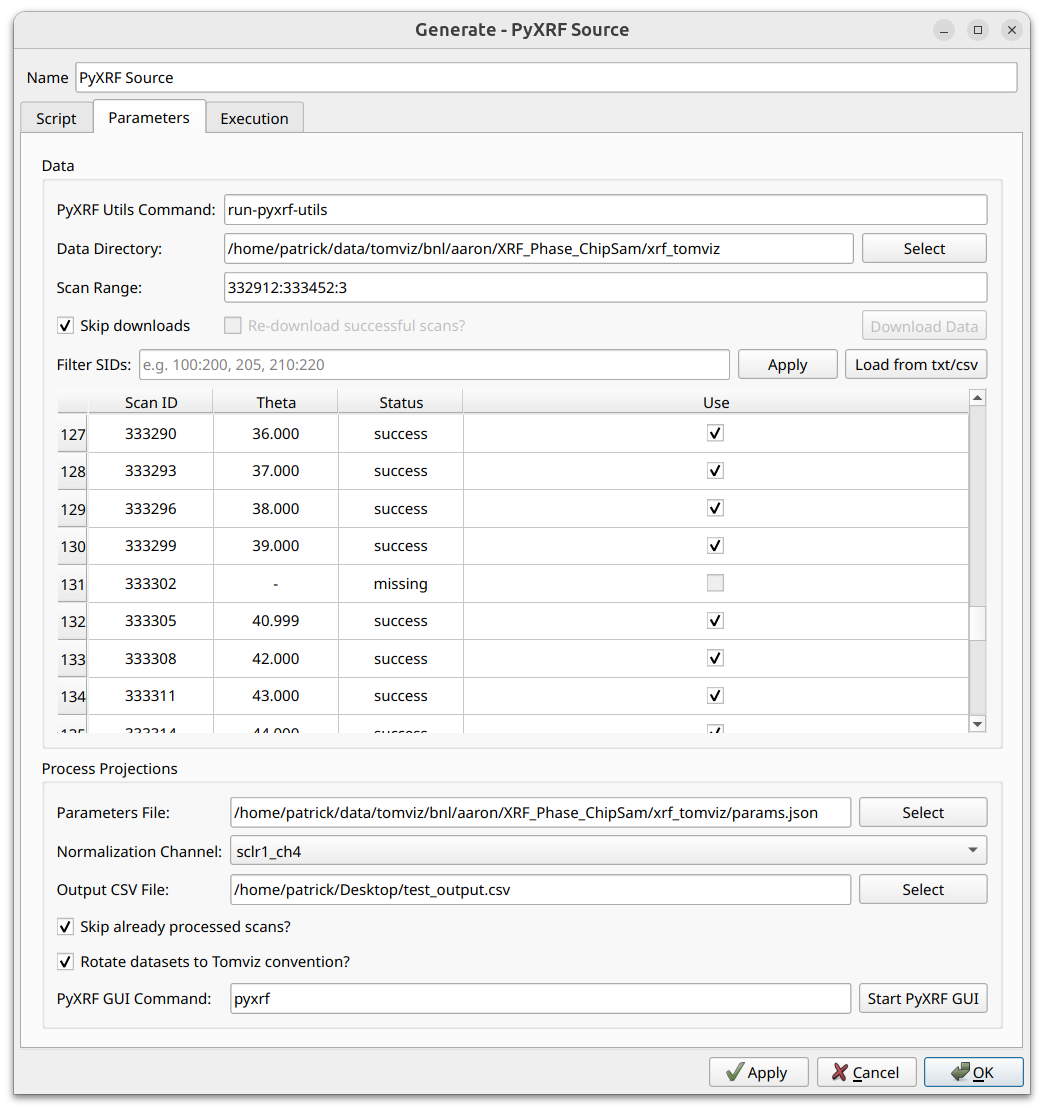
Data Download

The top section of the Parameters tab configures data downloading:

• PyXRF Utils Command - The command used to execute PyXRF utilities (e.g. run-pyxrf-utils). This can be a script that sets up and runs pyxrf-utils in a different environment. The command-line API is expected to match that shown here.

• Data Directory - The working directory where data and log files will be stored. Click Select to browse.

• Scan Range - The range of scans to download, specified in start:stop:stride format (both start and stop inclusive).

• Skip downloads - When checked, skips the download step entirely and uses existing data on disk. This disables the Re-download successful scans checkbox and the Download Data button.

• Re-download successful scans? - When checked, re-downloads scans that were previously downloaded successfully.

Click Download Data to begin downloading. The scan table is populated automatically once the data directory contains scan data.

Scan Table

The scan table shows one row per scan with the following columns:

• Scan ID - The beamline scan identifier

• Theta - The tilt angle for this scan (shown as “-” for failed scans)

• Status - Download/processing status (success, fail, missing)

• Use - Checkbox to include/exclude this scan from processing (disabled for failed scans)

Filtering SIDs

The Filter SIDs field above the table supports numpy-like slice syntax for filtering displayed scans. Type a filter expression and click Apply. For example:

• 157394:157413:3 - Every third scan from 157394 to 157413

• 157394:157413:3, 157420:157500:2 - Comma-delimited multiple ranges

Filtered-out SIDs are hidden and excluded from subsequent processing.

SIDs can also be loaded from a text file or CSV file using the Load from txt/csv button. When loading a CSV, columns named “Scan ID” and “Use” are recognized, allowing you to reuse scan selections.

Processing Projections

The bottom section configures how the downloaded data is processed:

• Parameters File - The JSON parameters file created using PyXRF GUI. Click Select to browse, or use Start PyXRF GUI at the bottom to launch the GUI and create this file. Follow the official PyXRF Documentation for modeling and fitting elements.

• Normalization Channel - The ion chamber channel for normalization (auto-detected from data; typically sclr1_ch4 for HXN).

• Output CSV File - Optionally specify a CSV file path to write scan metadata. Click Select to browse.

• Skip already processed scans? - Skip HDF5 files that already contain processed results. Uncheck this if you changed the parameters file or normalization channel.

• Rotate datasets to Tomviz convention? - Rotate the resulting tilt image stacks to match the convention expected by reconstruction transforms.

• PyXRF GUI Command - The command to launch PyXRF GUI (default: pyxrf). Can be overridden with the TOMVIZ_PYXRF_EXECUTABLE environment variable.

• Start PyXRF GUI - Launches the PyXRF GUI for creating the parameters file.

Output

After processing, the extracted elements are loaded as a single tilt series source node in the pipeline, with each element as a separate scalar array. The voxel sizes are set automatically from the XRF data metadata when available.

XRF Data Analysis

After the source produces its output, the data appears in the pipeline as a tilt series with multiple arrays (one per element). The Properties panel shows the Active Scalars dropdown for switching between elements, and a Dimensions & Range table listing all scalar arrays with their data ranges and types.

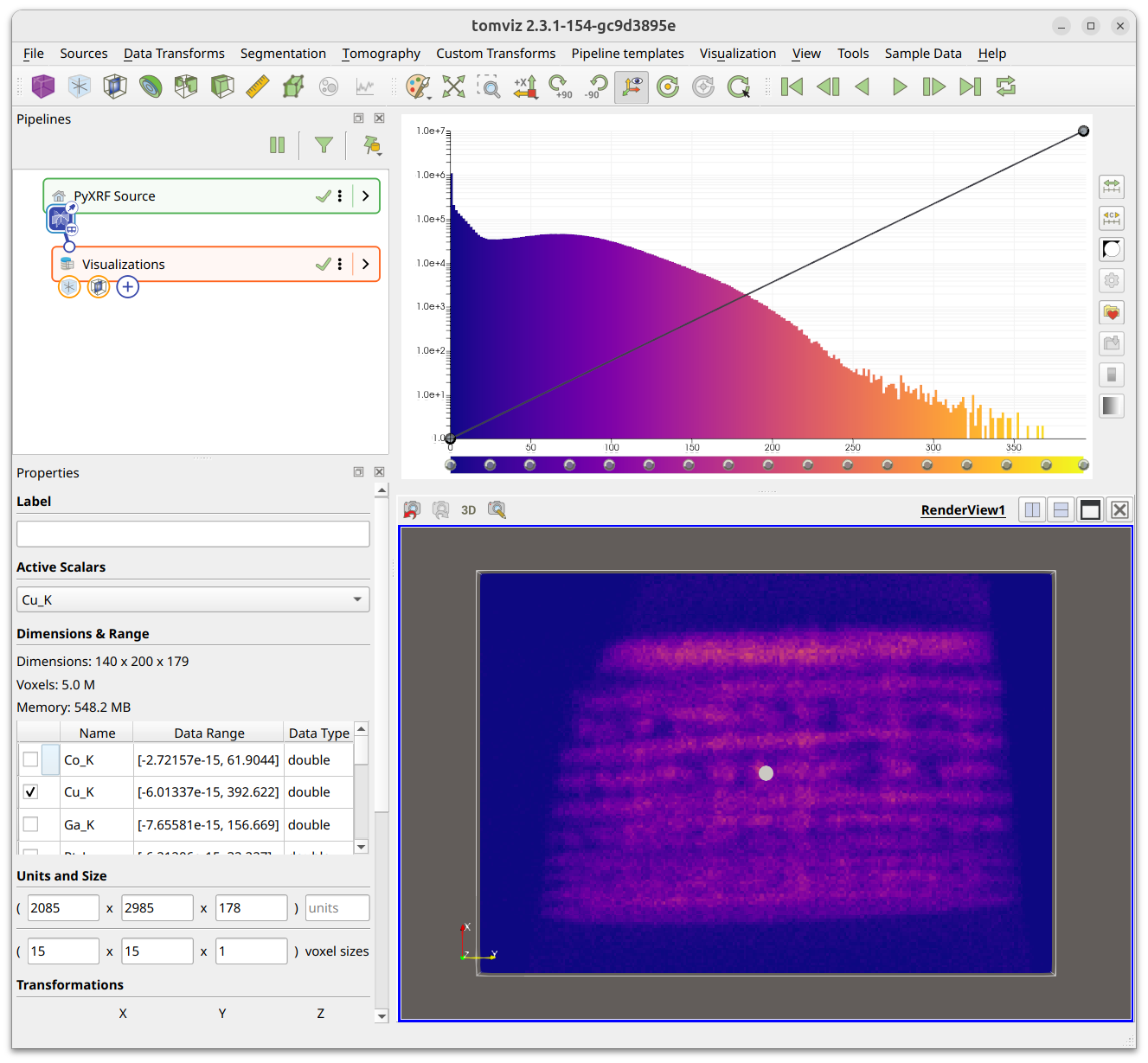
The currently “active” array can be switched to visualize different elements. This “active” array is also what is used by transforms as dataset.active_scalars, so make sure the correct array is selected before running a transform.

PyStackReg Image Alignment

A typical next step is to perform image alignment using the PyStackReg image alignment transform. Before opening the transform, first determine an ideal array (one with a high signal-to-noise ratio) and an ideal slice (close to 0 degrees, or close to the middle of the image). Select the ideal array as the active array, and navigate to the ideal slice in a slice visualization.

Then click Tomography > Alignment > Image Alignment (Auto: PyStackReg):

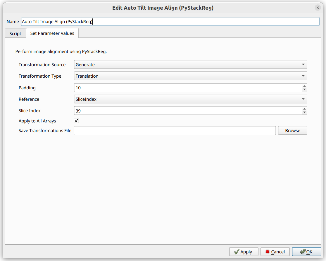
The transform defaults to selecting the Slice Index of the currently viewed slice. The PyStackReg transform determines transformation matrices using the currently selected active array and applies those same matrices to all arrays.

Select the Transformation Type (Translation is a good starting point). Padding can help ensure the image does not wrap around.

The option to Save Transformations File saves transformations and pixel sizes in NPZ format. These can be reused with the Load From File option on datasets with different pixel sizes (such as ptychography data).

More details about PyStackReg can be found in the alignment section.

Tilt Axis Shift Alignment

After PyStackReg alignment, center the data before reconstruction. Navigate to Tomography > Alignment > Tilt Axis Shift Alignment (Auto):

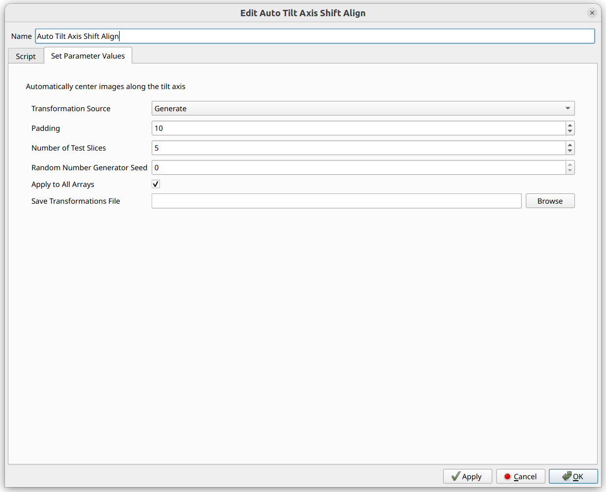
Options are similar to PyStackReg, including loading/saving shifts from/to files, padding, and applying to all arrays. The transform randomly selects slices to test for determining the ideal alignment.

More details about Tilt Axis Shift Alignment can be found in the alignment section.

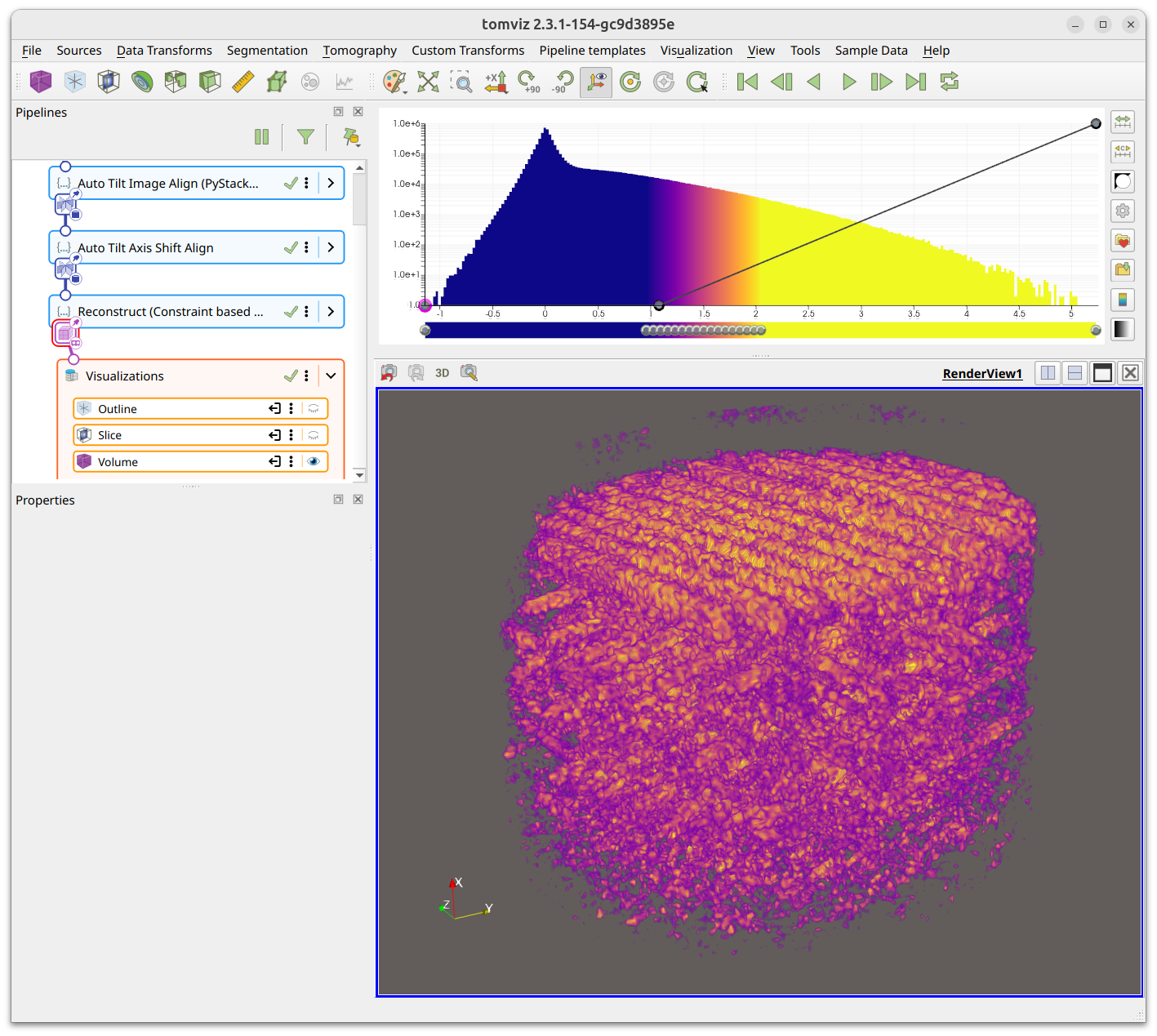
3D Reconstruction

After alignment and centering, perform a 3D reconstruction. The primary reconstruction transforms for the XRF workflow are the “Constraint-based Direct Fourier Method” and the “Direct Fourier Method”, available under Tomography > Reconstruction.

The reconstruction transform iterates through every array and performs the reconstruction on each one.

Once reconstruction finishes, the output appears downstream in the pipeline with Outline, Slice, and Volume visualizations. Adjust the opacity editor to highlight features of interest:

Different elements can be selected via the Active Scalars dropdown in the Properties panel.

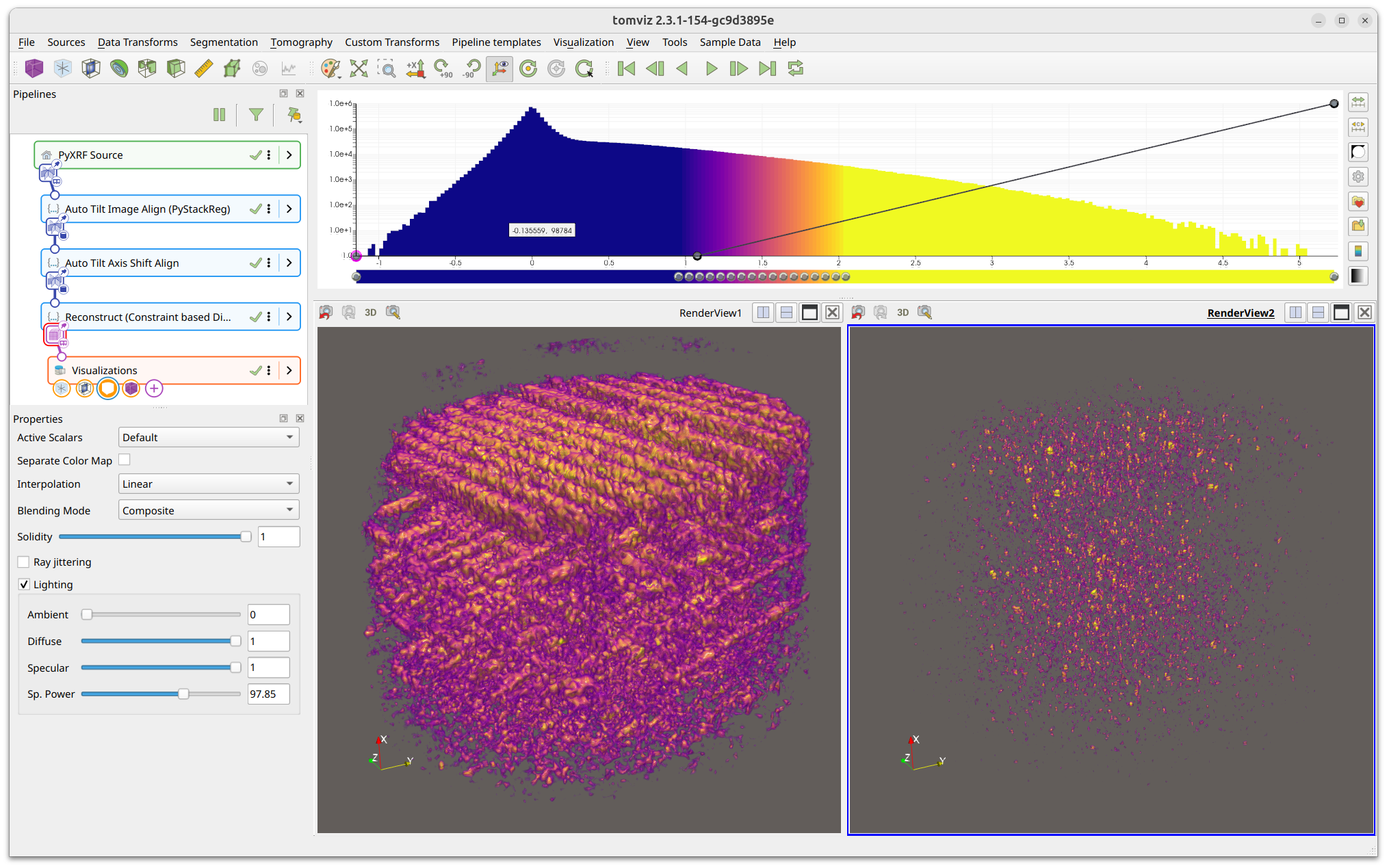
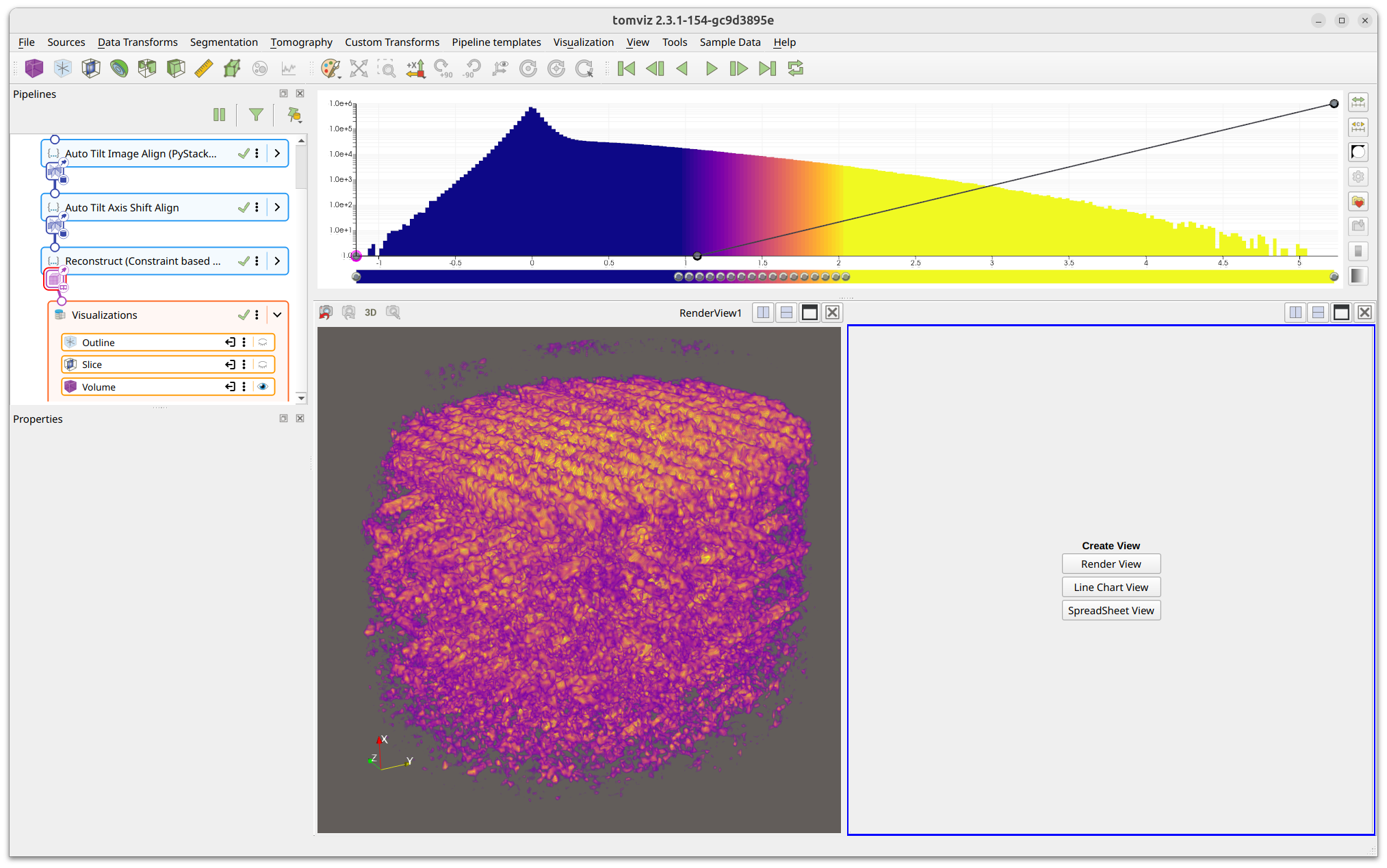
Comparatively Visualizing Different Elements

Multiple elements can be visualized simultaneously in separate render views. Click one of the split icons in the top-right section of the render window to divide the view area. A dropdown appears with view type options - select Render View:

Click on the new render view to select it (indicated by a blue border), and add a new Volume visualization. In the volume properties, change Active Scalars to a different element to compare side-by-side:

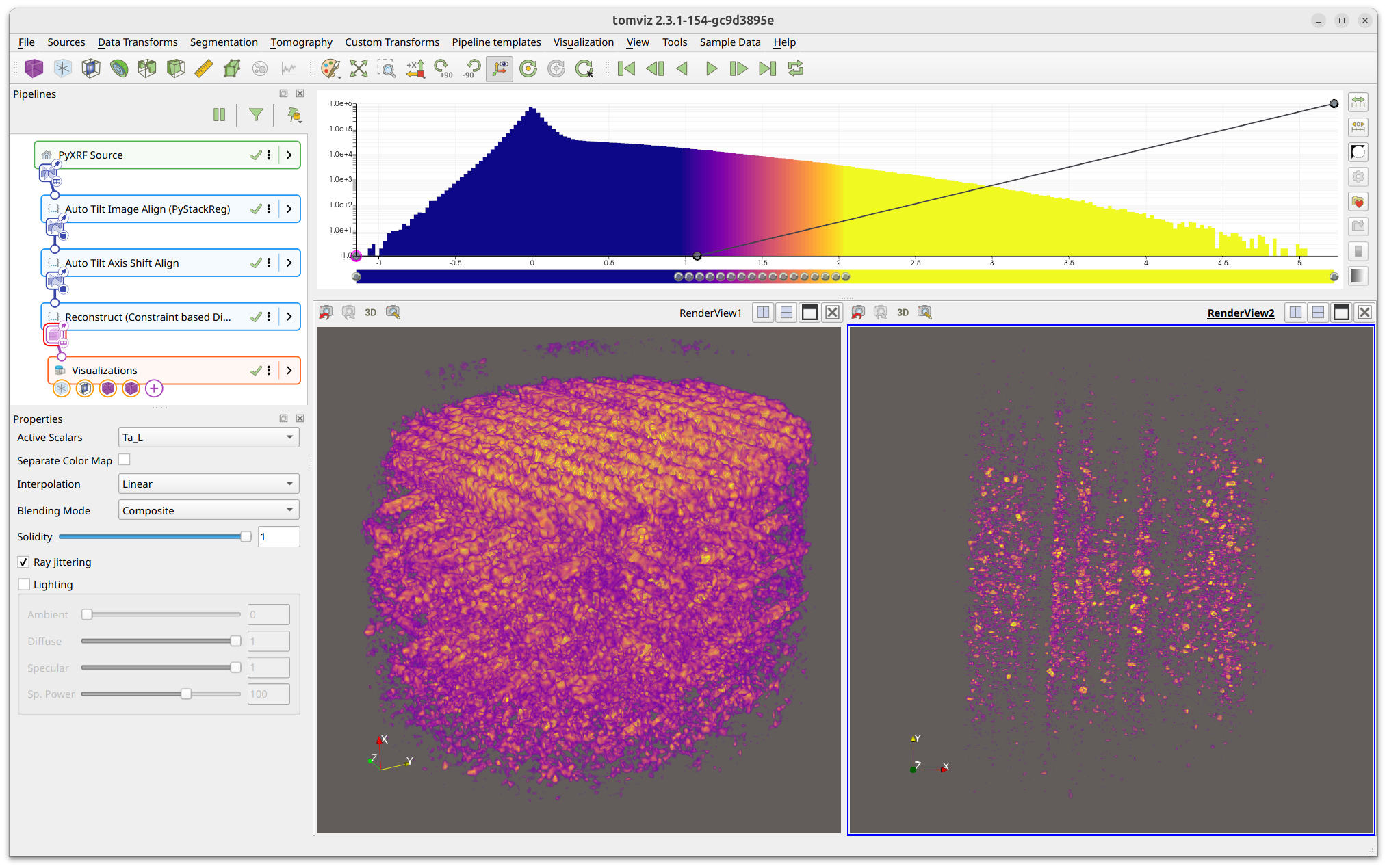
Link cameras between render views so they rotate together: right-click one view, click Add Camera Link, and then left-click the other view:

More realistic rendering can be achieved by enabling lighting in the volume properties and adjusting the Diffuse, Specular, and Specular Power sliders: