Ptycho Source
The Ptycho source streamlines the stacking and analysis of ptychography data, particularly for the HXN beamline at NSLS-II.
It relies on NSLS-II’s Ptycho GUI to download and process the ptycho data into a directory with pre-defined file paths. This directory is specified within the Ptycho source widget in Tomviz, which then automatically stacks, formats, and loads the data.
Steps for the subsequent data analysis of the Ptycho data are included in Tomviz, including deleting invalid slices, performing automatic image alignment, centering the images, performing the 3D reconstruction, and then comparatively visualizing different reconstructed elements. Those steps are also detailed below.
To begin, click on Sources in the top menu bar, and then select Ptycho.
Tutorial Video
Ptycho Source Widget
After selecting Sources > Ptycho, a source node is created in the pipeline
with a configure dialog containing Script, Parameters, and Execution tabs.
The Parameters tab contains the full data loading interface. All settings are
persisted between sessions.
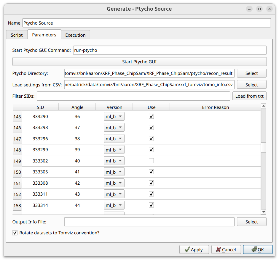
Ptycho GUI
If the ptycho data has not yet been downloaded and processed, specify the
command in the Start Ptycho GUI Command field (e.g. run-ptycho) and click
Start Ptycho GUI. See the
Ptycho GUI documentation for usage
instructions.
Directory Selection
Once the ptycho data has been processed, specify the output directory
containing the scan ID subdirectories (e.g., S157391, S157394) in the
Ptycho Directory field. Click Select to browse. Tomviz will automatically
analyze the directory and populate the scan table. If the directory contains a
recon_result subdirectory, it will be auto-detected.
Loading Settings from CSV
The Load settings from CSV field allows you to specify a CSV file to
automatically configure the scan table. Click Select to browse. CSV files
generated from the PyXRF source are compatible. When
loaded, the CSV file will:
Mark each SID as “Use” that was marked as “Use” in the CSV
Unmark SIDs missing from the CSV or not marked as “Use”
Set versions from the “Version” column if present
Filtering SIDs
The Filter SIDs field supports numpy-like slice syntax:
157394:157413:3- Every third SID from 157394 to 157413157394:157413:3, 157420:157500:2- Multiple comma-delimited ranges
SIDs can also be loaded from a text file using the Load from txt button.
Filtered-out SIDs are hidden and excluded from stacking.
Scan Table
The table shows one row per SID with five columns:
SID - The scan identifier
Angle - The tilt angle
Version - Combo box for selecting the reconstruction version (e.g.
ml_b). When multiple versions are available, use the dropdown to choose. Multiple rows can be selected and their versions set together via the context menu.Use - Checkbox to include/exclude this SID
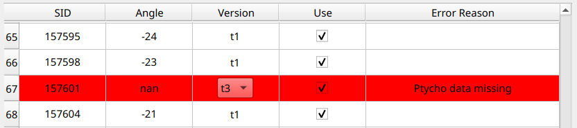
Error Reason - Displays any detected errors for this SID/version combination
If errors are detected for a particular SID and version combination, the row appears red with the error reason displayed:
Output Options
Output Info File - Optionally specify a text file to write a summary of the stacking configuration. Click
Selectto browse.Rotate datasets to Tomviz convention? - Rotate the resulting datasets to match the convention expected by reconstruction transforms
Output
When the source executes, it produces two tilt series datasets via two output ports on the Ptycho Source node (visible as two colored dots below the node in the pipeline strip widget):
object - Contains
AmplitudeandPhasearraysprobe - Contains
Probes AmplitudeandProbes Phasearrays
Analyzing Ptycho Data
After stacking and importing, the data appears in the pipeline with the Ptycho Source node showing its two output ports. Each port feeds into its own set of visualizations:
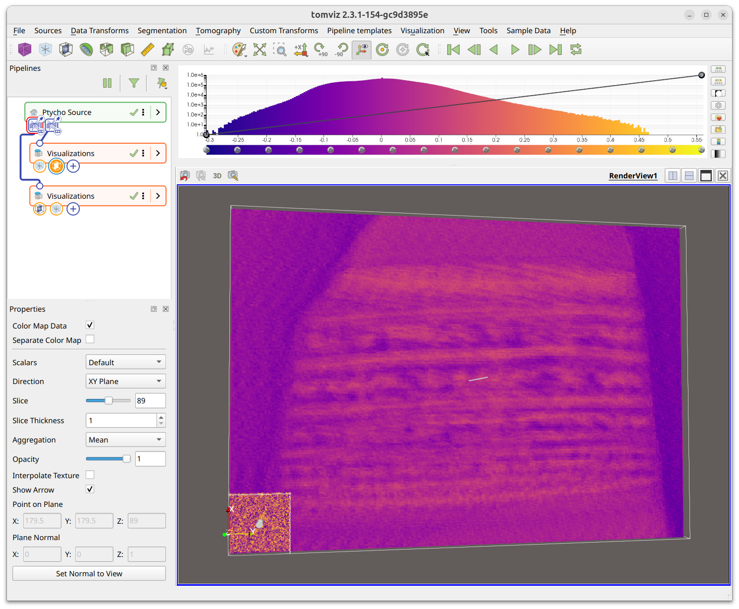
The probe slice may appear much smaller than the ptycho object because the voxel sizes differ (typically ~5 nm for the object vs ~1 nm default for the probe). If the probe is not needed, its visualizations can be deleted from the pipeline.
Select the ptycho_object and verify the voxel sizes in the Properties panel.
Correct voxel sizes are important if transformation matrices from the XRF
workflow will be applied to the ptycho dataset.
The Ptycho workflow then follows the same analysis steps as the XRF workflow, as outlined in the PyXRF data analysis section. If transformation matrices were saved during the PyXRF workflow, the same SIDs were used, and voxel sizes are correct for both datasets, the same transformation matrices can be applied to the ptycho data.
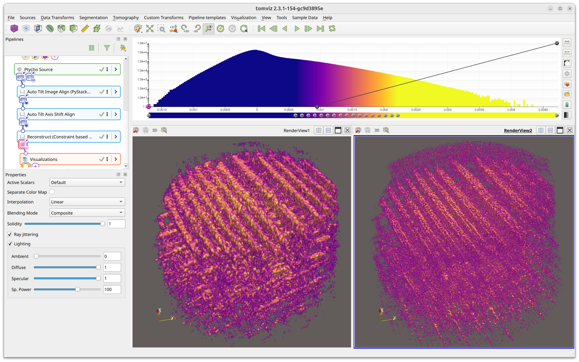
If voxel sizes are set properly for both XRF and Ptycho data, they can be visualized together and will appear approximately the same size. In the screenshot below, the left render view shows XRF data and the right shows ptychography data. The higher spatial resolution of ptychography is clearly visible in the finer structural detail.