Catalog

Tortuosity

The Tortuosity operator calculates various quantities described in the paper by Chen-Wiegart et al.

The operator can be found under the Data Transform menu.

Parameters

• phase (int): the scalar value in the dataset that is considered a pore

• distance_method (enum): the distance method to calculate distance between pore nodes. Options are: Eucledian, CityBlock, Chessboard.

• propagation_direction (enum): the face of the volume from which distances are calculated. Options are X+, X-, Y+, Y-, Z+, Z-.

• save_to_file (bool): save the detailed output of the operator to files. If set to True, propagate along all six directions and save the results, but only display results for one direction within the application.

• output_folder (str): the path to the folder where the optional output files are written to

Output

• Volumetric data: in the output volume are saved the distances between each pore voxel and the starting propagation face.

• Path length table: the average path length for a face vs the linear length

• Tortuosity table: 4 different tortuosity values calculated from the path length table.

• Tortuosity distribution table: the distribution of tortuosities for voxels in the last slice of the propagation

• If the save_to_file parameter is set to True, the quantities above will also be saved to disk inside output_folder for all the possible propagation directions. For each direction, the following files are created:

  • distance_map_*.npy

  • path_length_*.csv

  • tortuosity_*.csv

  • tortuosity_distribution*.csv

Pore Size Distribution

The Pore Size Distribution operator calculates the continuous pore size distribution as described in the paper by Münch and Holzer

The operator can be found under the Data Transform menu.

Parameters

• threshold (int): scalars greater than threshold are considered matter. scalars less than threshold are considered pore.

• radius_spacing (int): the pore size distribution is computer for all radii from 1 to r_max. Tweak the radius_spacing parameter to reduce the number of radii. For example, if radius_spacing is 3, only calculate distribution for r_s = 1, 4, 7, ... , r_max.

• save_to_file (bool): save the detailed output of the operator to files.

• output_folder (str): the path to the folder where the optional output files are written to

Output

• Volumetric data: for each pore voxel, save distance from the closest matter voxel.

• Pore size distribution table: the fraction of the total volume that can be filled by spheres with the a certain radius

• If the save_to_file parameter is set to True, the quantities above will also be saved to disk inside output_folder. The following files are created:

  • pore_size_distribution.csv

FXI Workflow

Running

The FXI Workflow operator uses tomopy to perform a reconstruction as needed in the Full Field X-ray Imaging workflow. The operator has a custom UI that allows the user to generate and visualize reconstructions of a single slice with different rotation centers, so that a reasonable rotation center for the full reconstruction may be chosen. Since both the operator and the UI require tomopy, the FXI Workflow operator may only be used if Tomviz was downloaded from conda-forge, and tomopy was installed in that conda environment.

The operator can be found under the Tomography menu.

To visualize reconstructions of a slice with different rotation centers, first set the various options in the Test Rotation Centers group and then click the Test Rotations button. This will run the test_rotations() function in the script with the selected parameters. After the reconstructions are generated, the left side of the dialog will display the reconstruction for the selected slice at the selected rotation. Use the Rotation slider bar in the Rotations Preview Settings group to scroll through and identify the rotation center with the clearest reconstruction. After a reasonable estimated rotation center is found, a more precise rotation center may be identified by narrowing the “Start” and “Stop” window, clicking Test Rotations, and scrolling through the reconstructions again. The colormap and Min/Max may also be edited to improve the contrast of the image.

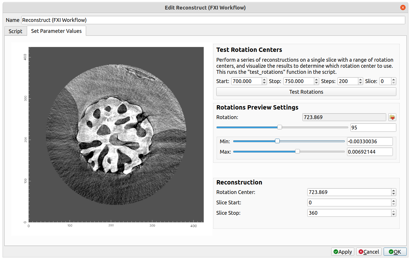
The settings for the reconstruction operation may be found in the Reconstruction group. If test rotations were visualized, the Rotation Center will automatically be set to match the rotation center of the current preview on the left side of the dialog. Select the start and stop slices, and then click OK. This will run the transform() function in the script with the selected parameters. A “Reconstruction” dataset will be created as the output, to which further processing and visualization can be performed. For the reconstruction of the example above, after performing a circle mask, followed by adding a “Volume” visualization module, and editing the color opacity histogram at the top of the application, the following is displayed:

Adding Custom Parameters

The FXI Workflow operator also allows custom parameters to be added to the UI, which will be passed to the relevant functions when they are called. Custom parameters for the reconstruction can be added as follows:

1. Save the FXI Workflow script by selecting the FXI Workflow operator, clicking on the Script tab, and clicking the Save Script button below the script. The name does not matter, but save it with a .py extension in the default directory that appears in order for Tomviz to automatically load it on start-up.

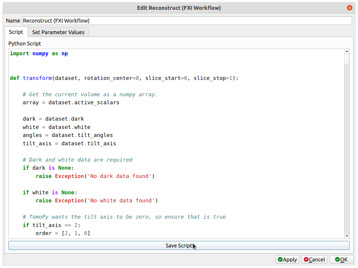
This will save both the script and a .json description file alongside it.

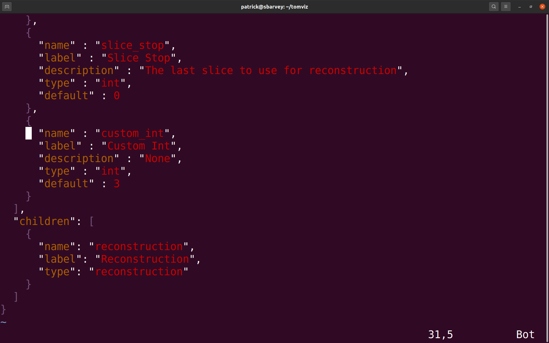
2. Navigate to the directory where the script was saved and open the .json file that was saved next to it (it should have the same name as the saved script except with a .json extension). In the parameters list, add a new parameter by following the example of the other parameters there (see detailed documentation of the .json file in Operator Development). The new parameter must have a unique name, and this name will be used as an argument in the transform() python function. See the custom_int parameter in the example below.

3. Save the .json file. Next, either click on Custom Transforms->Import Custom Transform... and select the python script, or restart Tomviz if the file was saved in its default directory. The operator should appear under the Custom Transforms menu. Select it. There should be a new group in the Reconstruction group named Additional Parameters, and the extra parameter with the provided label should be there. In this case, the extra parameter is “Custom Int”.

4. The new parameter needs to be added as an argument to the transform() function. Select the “Script” tab, find the transform() function, and add an argument with the same name as the newly added parameter (custom_int, in the above example). When “Apply” or “OK” is clicked, the operator will begin, and the extra parameter will be passed into the transform() function as that argument. Save the script one more time so that it includes the new argument.

In the FXI Workflow operator, new parameters may also be added to the Test Rotation Centers group, which will be passed to the test_rotations() function in the script. To do so, follow the same instructions as above, except that in the .json file, provide a tag key to the parameter with a value of test_rotations, like so:

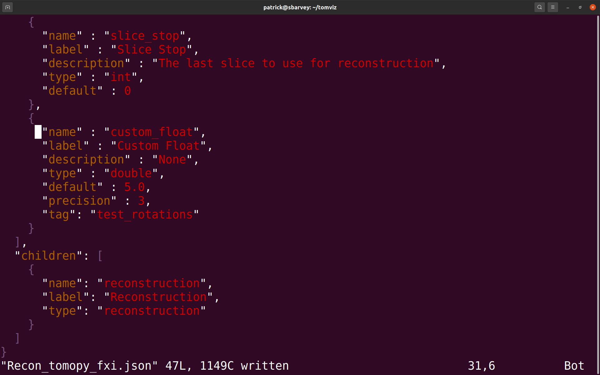
The added parameter should appear within the Test Rotation Centers group within a newly visible Additional Parameters group, like so:

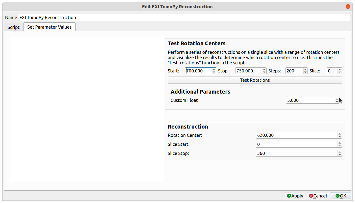
Select the “Script” tab, find the test_rotations() function, and add an argument with the same name as the newly added parameter (custom_float, in the above example). When “Test Rotations” is clicked, the extra parameter will be passed into the test_rotations() function as that argument. Save the script one more time so that it includes the new argument.

This process may be repeated to add any number of extra parameters to either the reconstruction operation or the “Test Rotations” feature.

Test Rotation Parameters

• Start (double): the starting value of the rotation centers to generate

• Stop (double): the final value of the rotation centers to generate

• Steps (int): the number of evenly spaced samples to generate over the [Start, Stop] interval

• Slice (int): the index of the slice to reconstruct using the rotation centers

Reconstruction Parameters

• Rotation Center (double): the rotation center to use for the reconstruction. If test rotations were previewed, this will automatically be set to match the current rotation center being previewed.

• Slice Start (int): the starting index of the slices to reconstruct (defaults to 0)

• Slice Stop (int): the final index of the slices to reconstruct (defaults to the last slice)

Output

• reconstruction: the reconstruction output

Manual Manipulation

The manual manipulation operator allows the user to visually manipulate a volume, and then apply those visual transformations to the underlying voxels. One use case is to manually register one volume with another.

Running

To perform manual manipulation, first ensure that the data source to be manipulated is selected in the pipeline view.

Next, select “Data Transforms” -> “Manual Manipulation”. The operator dialog should appear, and a red outline will be rendered in the view.

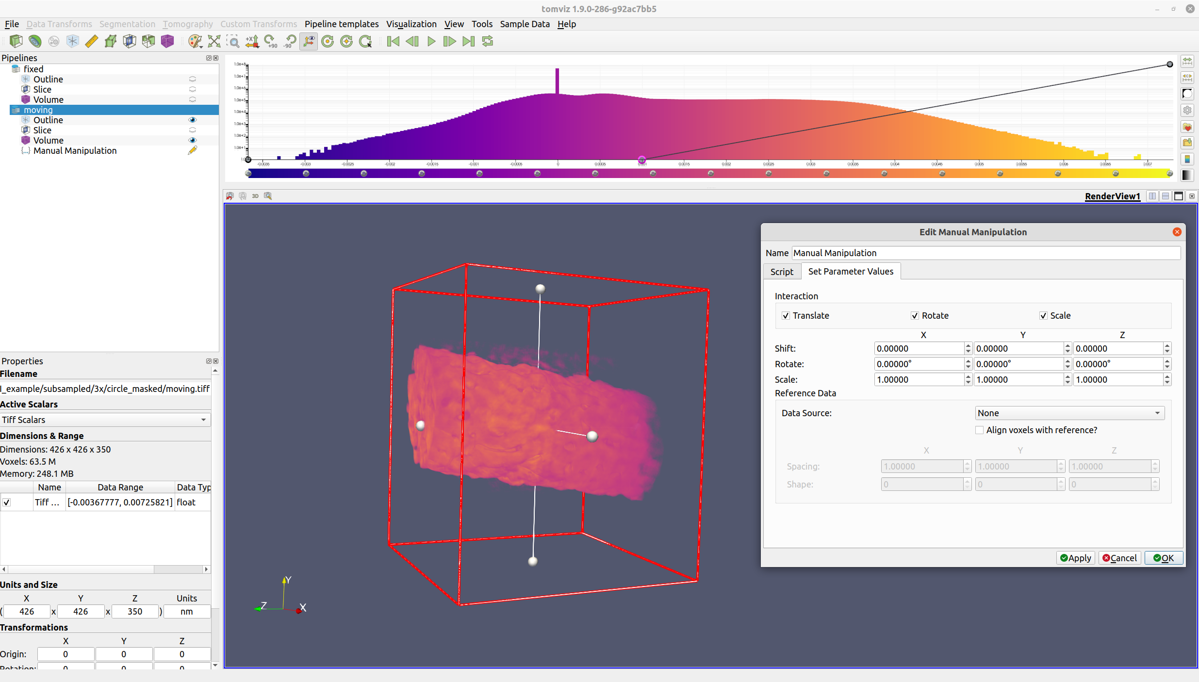
The red outline indicates the region where the voxels will lie after the operation has completed. Input voxels outside of this region will either be zeroed out (in the rotation step), or wrapped around to the other side (in the shift step).

All three types of interaction (translation, rotation, and scaling) may be enabled/disabled via their respective checkboxes. Translation may be performed by either middle-clicking and dragging the volume, or by left-clicking and dragging the middle handle. Rotation may be performed by left-clicking and dragging a face. Scaling may be performed by either left-clicking and dragging a face handle (for non-fixed aspect ratio scaling), or by right-clicking and dragging the volume (for fixed aspect ratio scaling).

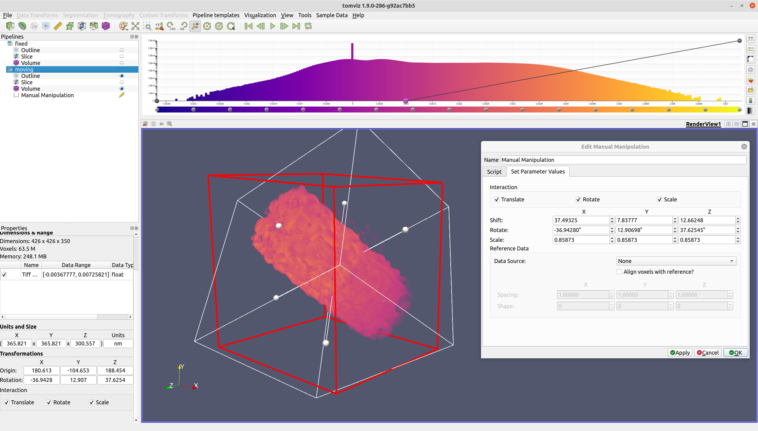
Once the volume is suitably transformed, click the “OK” button. The voxels will then be transformed via rotation, shift, and scaling.

The manual manipulation operator also provides the ability to assign a reference data source. If a reference data source is selected, the center of the reference data source will be moved to match the center of the moving data source. This is especially valuable if the data sources are different sizes, as it will allow for a more visually intuitive alignment.

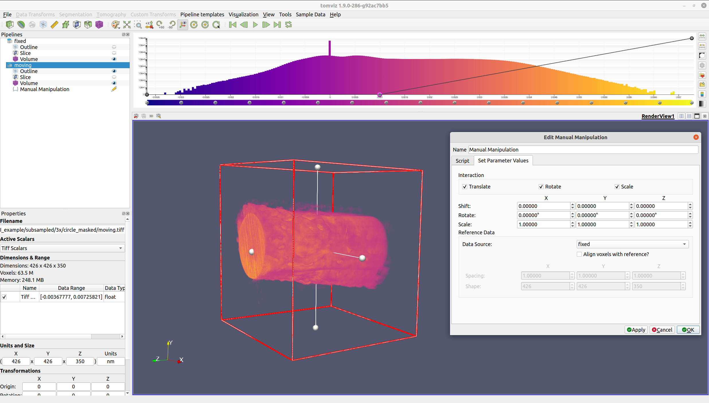
If “Align voxels with reference?” is checked, then the moving data source will be cropped, padded, and resampled so that the voxels align with the reference data source.

Alternatively, if “Align voxels with reference?” is checked, but the reference data source is “None”, the values of the reference spacing and shape may be entered manually. These values will then be used to determine the cropping, padding, and resampling that is needed.

Parameters

• Shift (int): the shift to apply to the voxels. In the custom Manual Manipulation widget, this is expressed instead as a double representing the shift in physical units. This is converted (including rounding) to integer shift. The shift is applied after rotation, and before any reference alignment.

• Rotate (double): the rotations to perform about the center of the volume in YXZ ordering (the same ordering that VTK uses internally). Rotation is performed before any other operation.

• Scale (double): the scaling to apply to the volume. This does not affect the voxels (unless “Align with Reference” is checked - see the “Reference Spacing” parameter for details). It is instead an attribute on the data source.

• Align with Reference (bool): whether to align the voxels of the output volume with a reference spacing and shape

• Reference Spacing (double): the reference spacing target. Resampling will be performed to transform the volume’s spacing to the reference spacing. This will only be applied if “Align with Reference” is True.

• Reference Shape (int): the reference shape target. Cropping/padding will be performed to transform the volume’s shape to the reference shape. This will only be applied if “Align with Reference” is True.

Output

• the resulting volume from the transformations

Deconvolution Denoise

The Deconvolution Denoise operator performs deconvolution-based denoising of volumetric data using a ptychographic probe and a selected regularization method. The operator uses the probe’s amplitude information as a point spread function (PSF) and applies deconvolution algorithms slice-by-slice along a chosen axis. This is particularly useful for denoising ptychographic reconstruction data by leveraging the known probe information.

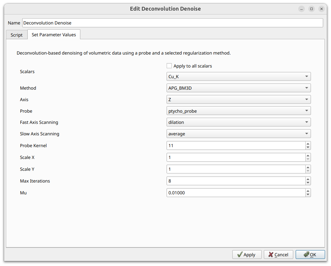
The operator can be found under the Data Transforms menu.

Methods

Three deconvolution methods are available:

• APG_BM3D (Accelerated Proximal Gradient with BM3D denoising): Generally the most accurate method, as BM3D is a state-of-the-art image denoising algorithm. However, it is the slowest of the three and requires the bm3d Python package, which is an optional dependency that must be installed manually into the Tomviz Python environment.

• APG_TV (Accelerated Proximal Gradient with Total Variation regularization): Uses total variation regularization within the proximal gradient framework. Does not require any additional dependencies.

• ADMM_TV (Alternating Direction Method of Multipliers with Total Variation regularization): A fast ADMM-based algorithm with TV regularization. Does not support upscaling (Scale X and Scale Y are disabled when this method is selected). Does not require any additional dependencies.

Parameters

• Scalars (select_scalars): which scalar arrays to process. If “Apply to all scalars” is unchecked, only the selected scalars will be denoised.

• Method (enum): the deconvolution method to use. Options are: APG_BM3D, APG_TV, ADMM_TV.

• Axis (enum): the axis along which to process slices. Options are: X, Y, Z.

• Probe (dataset): the probe dataset used for deconvolution. The operator looks for a scalar array with “amplitude” in its name within this dataset to use as the PSF.

• Fast Axis Scanning (enum): the scanning method for the fast axis. Options are: dilation, average.

• Slow Axis Scanning (enum): the scanning method for the slow axis. Options are: dilation, average.

• Probe Kernel (int): the size of the probe kernel extracted from the center of the probe amplitude. Default: 11.

• Scale X (int): X scale factor for super-resolution (only available for APG_TV and APG_BM3D methods). Default: 1.

• Scale Y (int): Y scale factor for super-resolution (only available for APG_TV and APG_BM3D methods). Default: 1.

• Max Iterations (int): maximum number of iterations. Default: 8.

• Mu (double): the mu regularization parameter. Default: 0.01.

Output

• The denoised volumetric dataset, with the same scalar arrays that were selected for processing. Scalars that were not selected are removed from the output. Scan IDs and tilt angles are preserved for matching slices.

Similarity Metrics

The Similarity Metrics operator computes similarity metrics between the current dataset and a reference dataset, producing a table of per-slice MSE (Mean Squared Error) and SSIM (Structural Similarity Index) values. This is useful for quantitatively evaluating the effect of processing steps such as denoising, by comparing a processed dataset against its original or a reference.

The operator can be found under the Data Transforms menu.

The results are output as a spreadsheet table which can be visualized as interactive line charts using the Plot module. Each selected scalar array produces two columns in the output: one for MSE and one for SSIM.

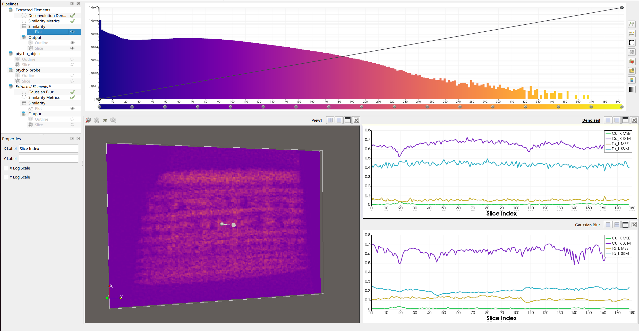
In the example above, the top-right plot shows the similarity metrics for a denoised dataset compared to the original. The SSIM values are closer to 1, indicating that the denoising successfully preserved structural similarity. The bottom-right plot shows the metrics for a Gaussian-blurred dataset compared to the original, where the SSIM values are noticeably lower, confirming that blurring degrades structural similarity more than the deconvolution denoising.

Parameters

• Scalars (select_scalars): which scalar arrays to compute metrics for.

• Axis (enum): the axis along which to process slices. Options are: X, Y, Z.

• Reference Dataset (dataset): the reference dataset to compare against. The operator matches slices between the two datasets using scan IDs when available, and resizes slices to a common size before computing metrics. Both slices are normalized to [0, 1] before comparison. If the reference dataset does not have a matching scalar name, the operator falls back to using a scalar array with “phase” in its name.

Output

• Similarity table: a spreadsheet with columns for the slice index, and for each selected scalar, a pair of MSE and SSIM columns. Lower MSE values indicate greater similarity, while SSIM values closer to 1.0 indicate higher structural similarity. The table can be visualized as line charts using the Plot module, or exported as CSV by right-clicking the result in the pipeline and selecting Export Table as CSV.

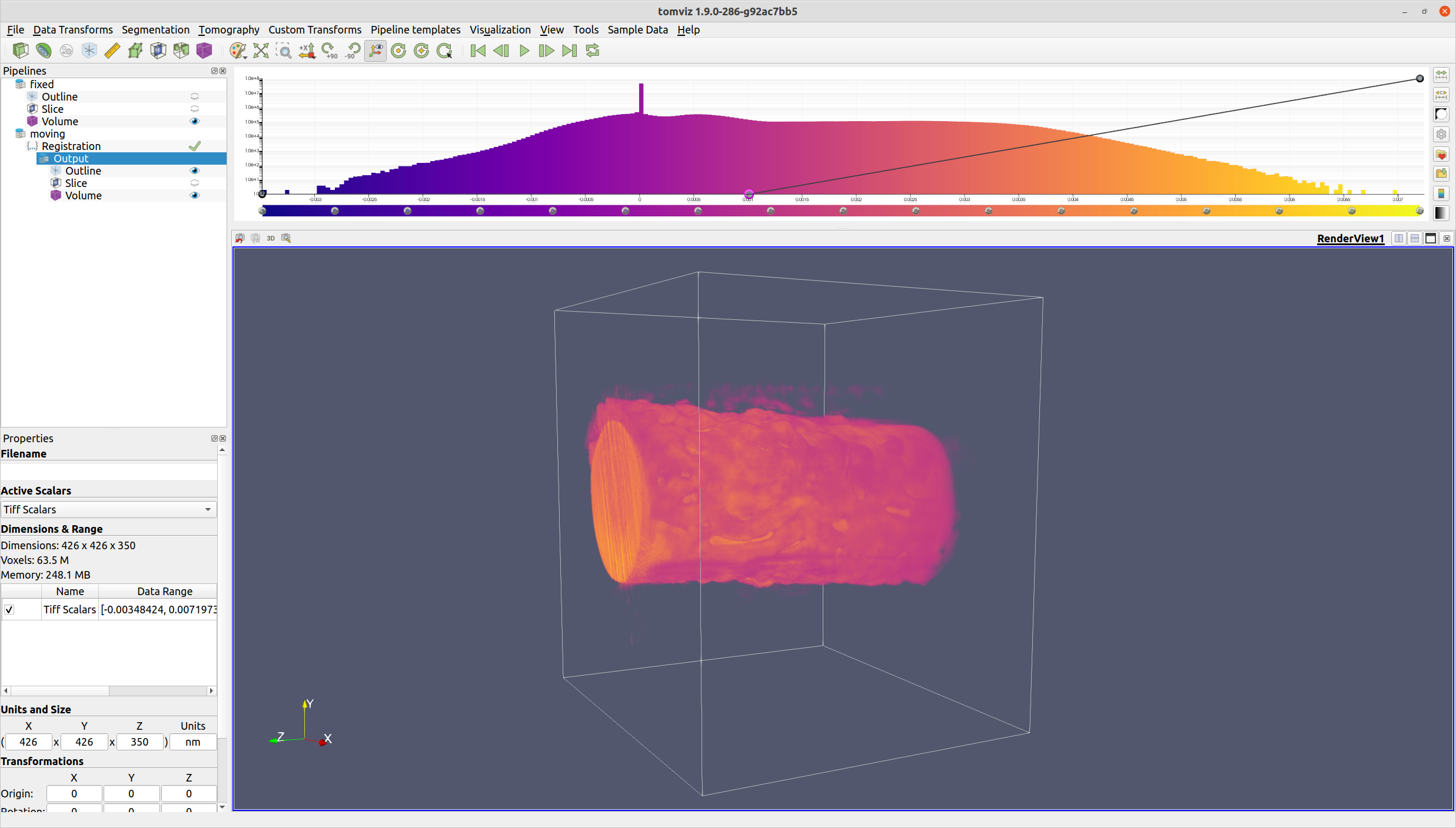
Registration

The registration operator may be used to automatically align one volume with another via voxel transformations. The transformation that is performed is rigid; it consists only of a translation and rotation.

Setup

This operator requires ITK Elastix, which is currently not being bundled with tomviz. As such, ITK Elastix must be installed in the tomviz python environment manually. This is possible if tomviz was installed from conda-forge or built locally.

ITK Elastix has wheels on PyPI, which were designed to work correctly within conda environments. Thus, whether tomviz was installed via conda-forge or built locally, running pip install itk-elastix should install it correctly. This may also upgrade the environment’s ITK libraries via PyPI, which should work fine as well.

Running

To perform registration, first ensure that the data source to be registered is selected in the pipeline view.

Next, select “Data Transforms” -> “Registration”. The operator dialog with the various options should appear.

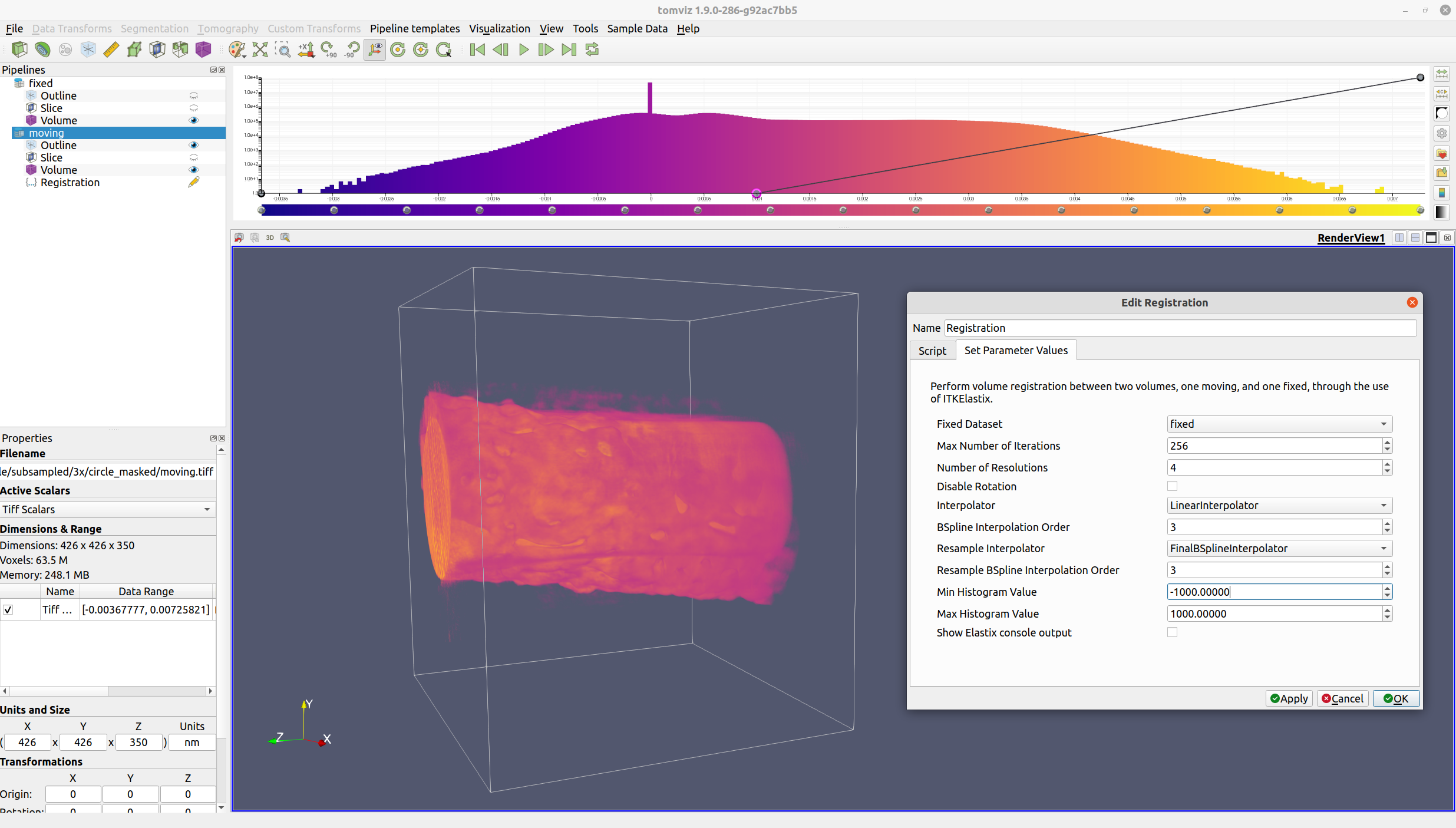
Ensure that the Fixed Dataset is set correctly to the fixed volume, and modify the various options as needed. Click “OK”, and registration will be performed.

ITK Elastix ensures that the output voxels will be aligned with the reference voxels.

Parameters

• Fixed Dataset (bool): the reference volume to which the input volume should be registered.

• Max Number of Iterations (int): the maximum number of iterations for ITK Elastix to use in each resolution.

• Number of Resolutions (int): the number of resolutions for ITK Elastix to use.

• Disable Rotation (bool): whether to perform a translation-only registration.

• Interpolation (enum): The interpolator that is used during optimization. Valid options are: NearestNeighborInterpolator, LinearInterpolator, BSplineInterpolator, and BSplineInterpolatorFloat.

• BSpline Interpolation Order (int): the order of the B-spline polynomial (only used if a BSpline interpolator is selected).

• Resample Interpolator (enum): The interpolator that is used to generate the final result. Valid options are: FinalNearestNeighborInterpolator, FinalLinearInterpolator, FinalBSplineInterpolator, and FinalBSplineInterpolatorFloat.

• Resample BSpline Interpolation Order (int): the order of the resample B-spline polynomial (only used if a resample BSpline interpolator is selected).

• Min Histogram Value (double): the threshold below which voxels will be masked out before performing registration. This may be used to mask out noise.

• Max Histogram Value (double): the threshold above which voxels will be masked out before performing registration. This may be used to mask out noise.

• Show Elastix console output (bool): whether or not to display the console output from Elastix.

Output

• the resulting volume from the registration